论文题目：Explore More Guidance: A Task-aware Instruction Network for Sign Language Translation Enhanced with Data Augmentation

发表会议：North American Chapter of the Association for Computational Linguistics (NAACL 2022)

第一作者：Yong Cao (PhD in HUST)

Question

如何解决 Sign Language Gloss Translation (SLGT) 的数据缺乏和 gloss 与 sentence 的表征空间不同的问题

Method

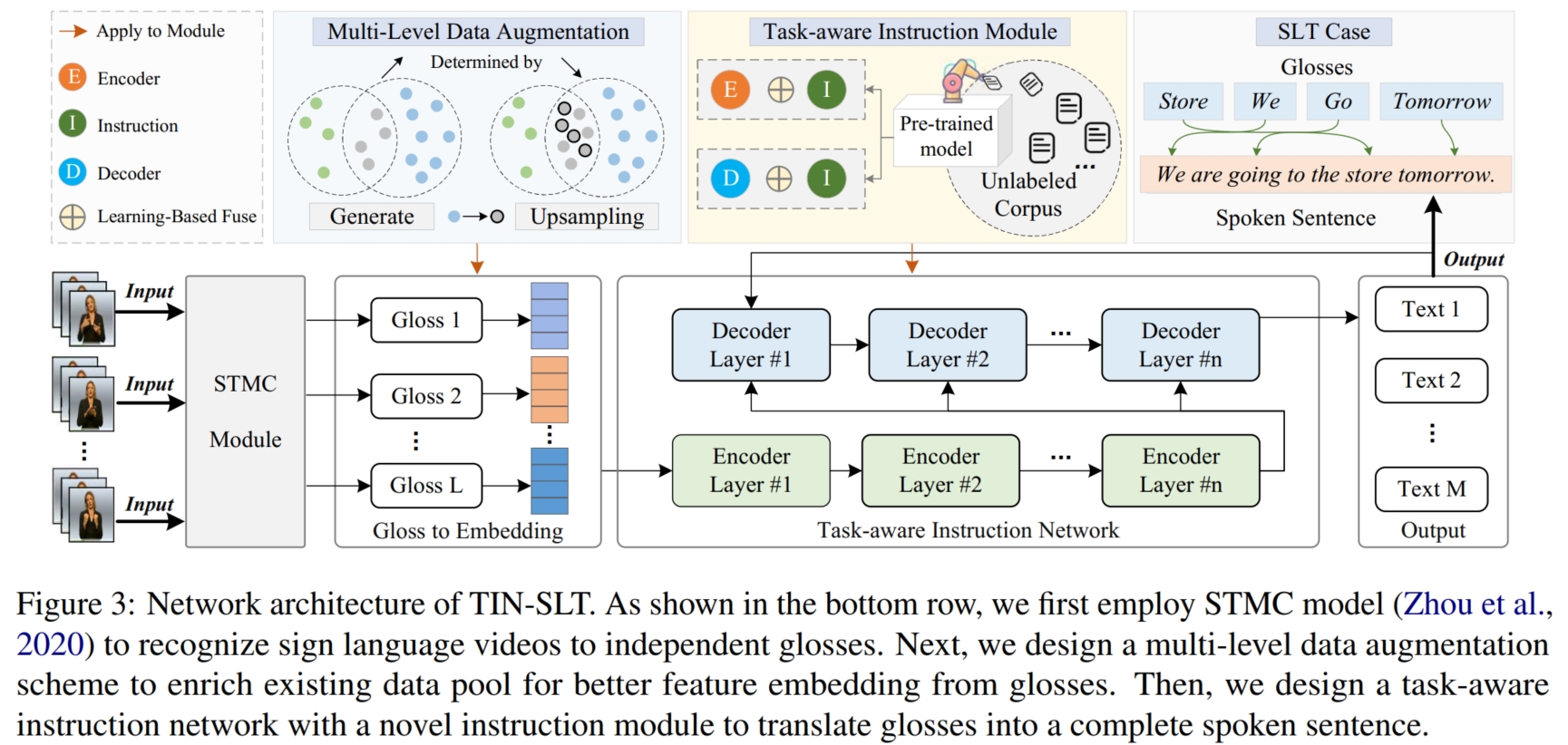
在如今大模型的时代下，最常见，也是最有效的解决数据缺乏的方法之一便是借助预训练的大模型。 如上图，本文便是将大模型编码得到的 embeddings 作为辅助信息使得模型能够学习到大模型的编码性能。 同时，为了解决表征空间差异问题，本文使用简单的上采样方法进行数据增强将 gloss 对齐到 sentence 空间。

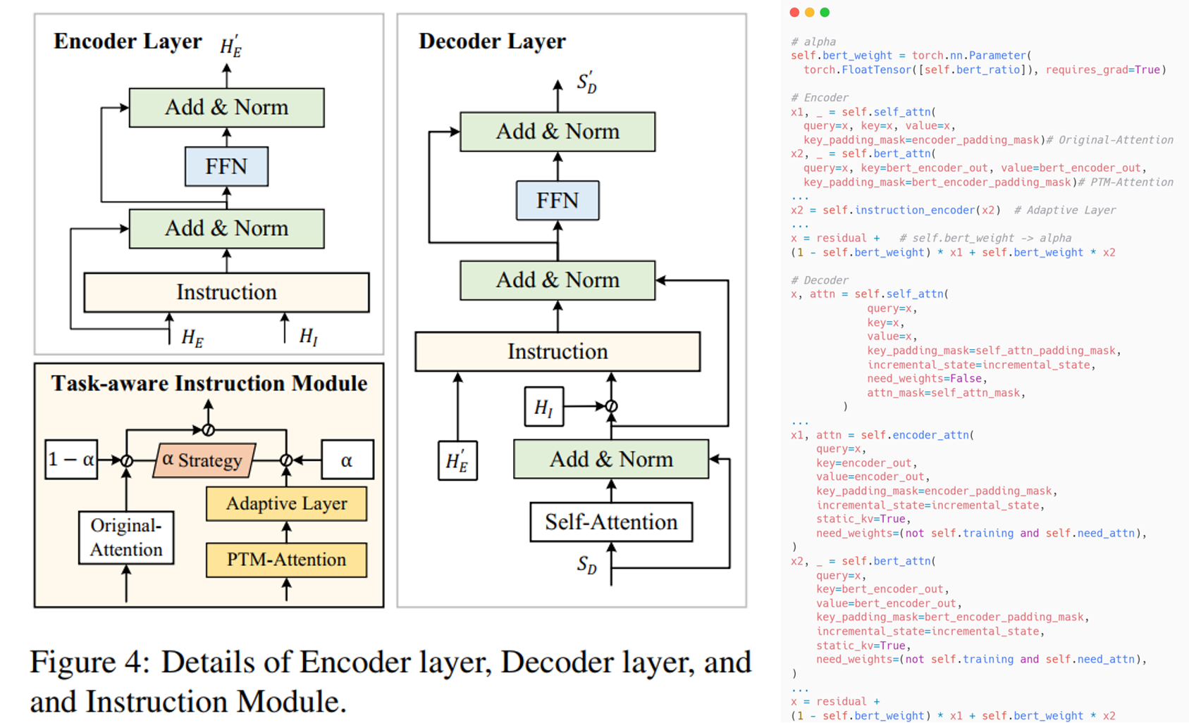
具体而言，如上图，本文使用的整体框架是 Transformer 的 Encoder-Decoder 框架。 假设数据集为 $D_o$，其中输入为 $\mathcal{G} = \{g_1,...,g_L\}$，输出为 $\mathcal{S} = \{\mathcal{w}_1,...,\mathcal{w}_M\}$。 为了将大模型的编码性能迁移到自身模型，本文提出了一个 Target-aware Instruction (TIM)模块嵌入 Encoder 和 Decoder 来帮助模型更好地学习。 TIM 的整体框架如图，包括一个 Original-Attention，一个 PTM-Attention，一个 Adaptive Layer 和一个 $\alpha$ 融合策略。 它包括 $3$ 个输入 $H_1$，$H_2$ 和 $H_3$，其中，$H_1$ 和 $H_2$ 是模型内部学习到的特征， 经过 Original-Attention (是一个 Cross-Attention)进行内部信息交叉学习更新：$\hat{h}_t^1 = Attn_O(h_t^1,H_2,H_2), H_1 = [h_1^1,...,h_T^1], \hat{H}_1 = [\hat{h}_1^1,...,\hat{h}_T^1]$。 而 $H_3$ 是外部的辅助信息(即大模型编码生成的 embeddings)，经过 PTM-Attention (也是一个 Cross-Attention)进行外部信息交叉学习更新， 然后使用 Adaptive Layer (本文使用一个线性层) 对更新后的特征进行进一步更新学习， 使其学习到 target-aware 的特征：$\hat{h}_t^3 = \sigma(Attn_P(h_t^1,H_3,H_3)), \hat{H}_3 = [\hat{h}_1^3,...,\hat{h}_T^3]$。 最后使用 $\alpha$ 融合策略将二者进行融合输出更新的 $\bar{H}_1$：$\bar{H}_1 = (1 - \alpha) \times \hat{H}_1 + \alpha \times \hat{H}_3$。

在 Encoder 中，假设 $H_I$ 为大模型编码生成的 embeddings，$H_E$ 和 $H_E'$ 分别为 Encoder 的输入和输出。 本文将原本的 MHA 替换成了 TIM，且 TIM 中的 $H_1 = H_E, H_2 = H_E, H_3 = H_I$ (即Encoder 的 TIM 的 Original-Attention 是 Self-Attention)， 然后 TIM 输出得到的 $\bar{H}_1$ 再经过一个 FFN 和 两次 Add & Norm 生成输出 $H_E'$：

在 Decoder 中，假设 $S_D$ 和 $S_D'$ 分别为 Decoder 的输入和输出。 本文将原本的 cross-MHA 替换成了 TIM。首先，输入 $S_D$ 经过一个 Mask-MHA，生成 $\tilde{S}_D$：

然后经过 TIM，TIM 中的 $H_1 = \tilde{S}_D, H_2 = H_E', H_3 = H_I$。 接着 TIM 输出得到的 $\bar{H}_1$ 再经过一个 FFN 和 两次 Add & Norm 生成输出 $S_D'$：

如上图右边代码，对于融合系数 $\alpha$，本文采用模型自我学习的方式，即将 $\alpha$ 设置为可学习的参数，随着模型的训练逐步更新。

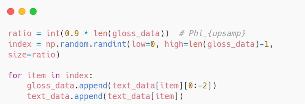
为了解决表征空间差异问题，本文使用上采样进行数据增强，并实现将 gloss 对齐到 sentence 空间。 具体而言，如上图代码，本文通过设置一个阈值 $\Phi_{upsamp}$，使用概率选择在优质候选数据集 $\mathcal{C}$ 中进行随机选择，生成一个新数据集 $D_n$：

该新数据集中的输入和输出数据均为 sentence，则就使得模型学习 gloss 和 sentence 的空间对齐。 同时为了获得合适的阈值 $\Phi_{upsamp}$，本文综合考虑数据集 $D_o$、数据 $\mathcal{G}^i/\mathcal{S}^i$ 和数据元素 $g_i/\mathcal{w}_i$ 的差异来进行抉择。 具体而言，本文考虑了四方面的因素：

• Token Level 1：Vocabulary Difference Ratio (VDR, $\phi_v$)，用来测量 gloss 和 sentence 的字典空间的差异性：

  $\phi_v = 1 - \dfrac{|W_\mathcal{G}|}{|W_\mathcal{G} \bigcup W_\mathcal{S}|}$

  其中，$W_\mathcal{G}$ 和 $W_\mathcal{S}$ 分别表示 gloss 和 sentence 的字典集。$|·|$ 表示大小。

• Token Level 2：Rare Vocabulary Ratio (RVR, $\phi_r$)，用来测量 gloss 中的生僻词的比例：

  $\phi_r = 1 - \dfrac{\sum_{\mathcal{G} \in W_{\mathcal{G}}} U(Counter(\mathcal{G}) < \tau_r)}{|W_\mathcal{G} \bigcup W_\mathcal{S}|}$

  其中，$U(·)$ 表示 $1$ 如果内部表达式为真，反之则为 $0$。$Counter(\mathcal{G})$ 表示 $\mathcal{G}$ 的出现频率。

• Sentence Level 1：Sentence Cover Ratio (SCR, $\phi_s$)，用来测量总体 gloss-sentence 对的相似性：

  $r_i = \dfrac{|\mathcal{G}_i \bigcap \mathcal{S}_i|}{|\mathcal{S}_i|},\ \phi_s = 1 - \dfrac{1}{N}\sum_{i, r_i > \tau_c}r_i$

  其中，$r_i$ 表示 gloss-sentence 对 $\{\mathcal{G}_i, \mathcal{S}_i\}$ 的相似性。 $\tau_c$ 表示 相似度阈值。此外，我们将所有相似度大于阈值 $\tau_c$ 的数据作为上采样的候选数据 $\mathcal{C}$。

• Dataset Level 1：Dataset Length-difference Ratio (DLR, $\phi_d$)，用来测量总体 gloss-sentence 对的长度差异：

  $\phi_d = 1 - \dfrac{\sum_i{|\mathcal{G}_i|}}{\sum_i{|\mathcal{S}_i}|}$

最后，使用不同的比例 $\theta = [0.1,0.1,0.6,0.2]$ 来对这 $4$ 个指标进行加权， 生成最后的阈值 $\Phi_{upsamp} = \theta * [\phi_v,\phi_r,\phi_s,\phi_d]$，并使用上采样算法(公式 $(1)$)对 $\mathcal{C}$ 进行采样生成数据集 $D_n$。 最后将原始数据集 $D_o$ 和生成数据集 $D_n$ 进行合并，一起作为数据集对模型进行训练。