这篇博客主要讲解关于 RLHF 的基础知识和训练 LLM 的具体(简易)代码实现.

RLHF 的基本原理

首先，RLHF 分为 $3$ 个部分：预训练 LLM 模型 $M_\theta$ ；预训练奖励模型 $r_\theta$ 以及 使用 PPO 微调 $M_\theta$.

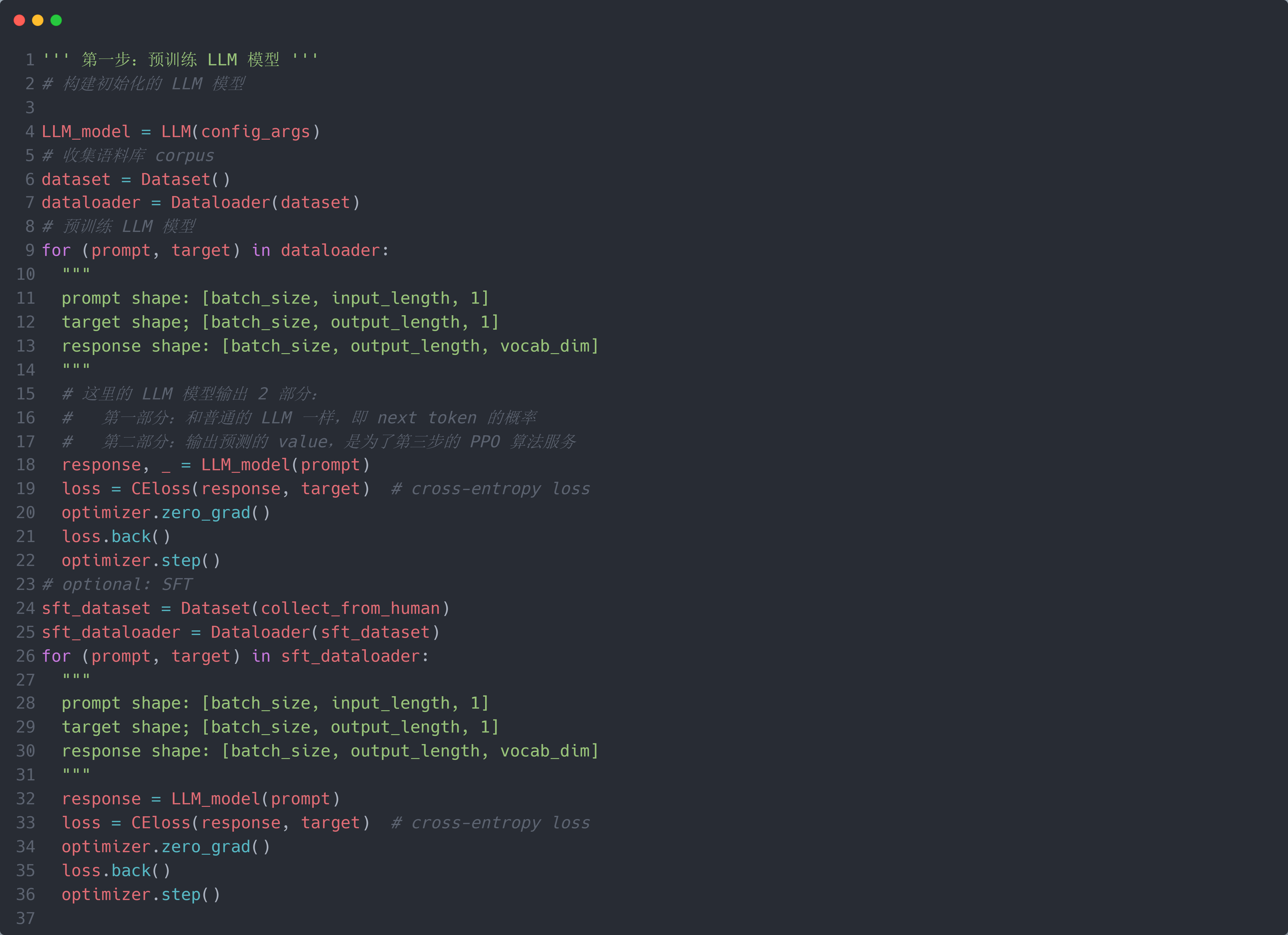
第一步：预训练 LLM 模型 $M_\theta$ (就是一个 Transformer Decoder 减去 cross-attention)：$M_\theta$ 输入一个 prompt (即输入的文本) $x \in \mathbb{R}^{L_I \times 1}$, 输入一个 response (即输出的文本) $y \in \mathbb{R}^{L_O \times 1}$. 和正常的预训练 LLM 过程一样，收集大量的文本数据(称为语料库 corpus)，使用 predict-next-token 的方式进行预训练 LLM 模型 $M_\theta$. 在预训练完成后，为了模型 $M_\theta$ 在第 $3$ 步有一个更好的初始化基础，可以再收集一些经过人为标注高质量的 Q & A 数据进行微调，称为 SFT (Supervised Fine Tuning).

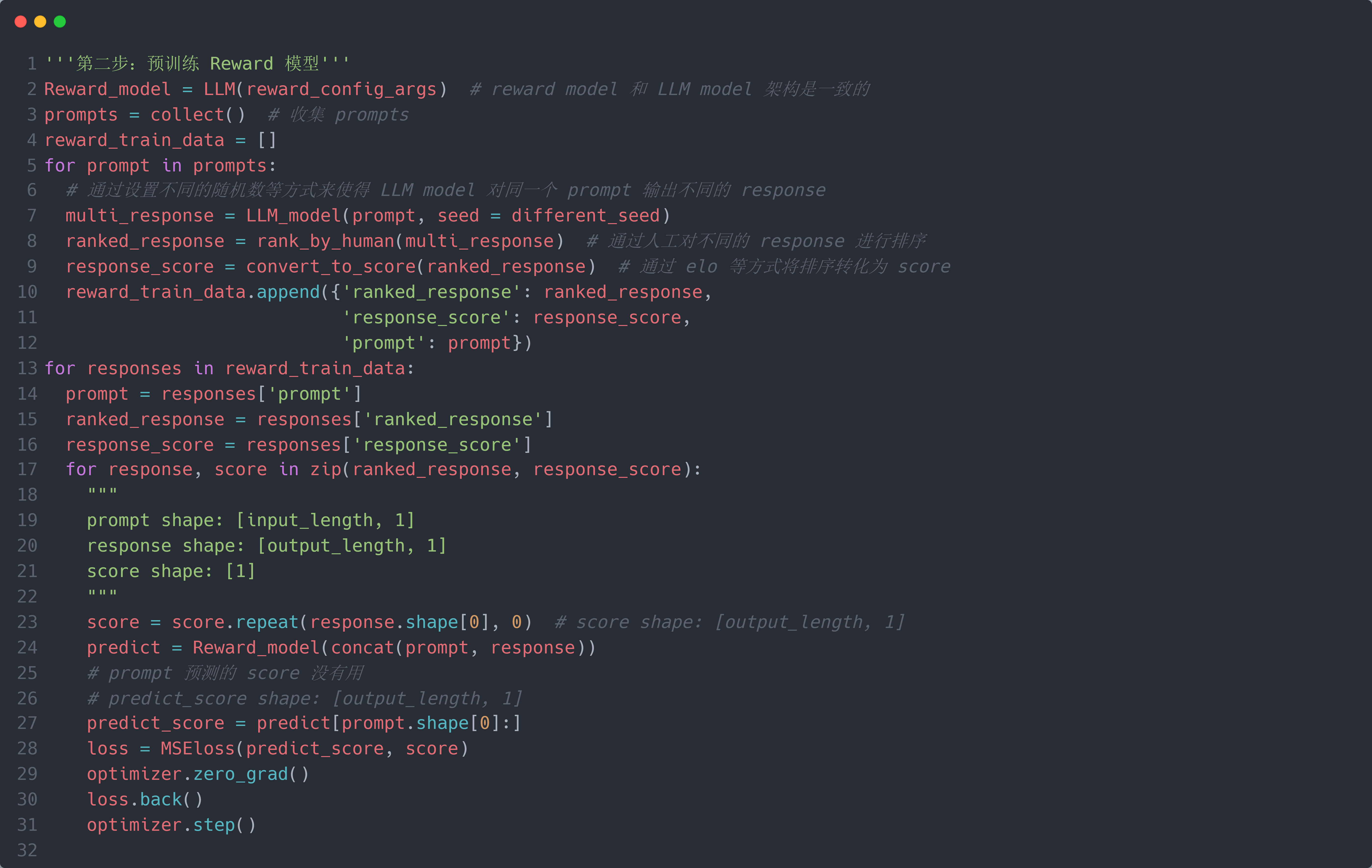
第二步：预训练奖励模型 $r_\theta$ (和 $M_\theta$ 一样的架构)：它的作用是根据人类的喜好对 $M_\theta$ 的输出进行打分(score)，这一步就是需要人工标注的步骤. 具体而言，给定 prompt $x$，LLM 模型 $M_\theta$ 输出 $y$，通过人工标注该输出的得分(score $s_{GT} \in R^{1 \times 1}$)作为 groud-truth (GT)；然后将两者进行拼接得到 $r_\theta$ 的输入，即 $r_\theta$ 的输入为 $\theta$ 的输入 + 输出 $z = concat(x, y) \in \mathbb{R}^{(L_I + L_O) \times 1}$, 输出每个词的 score (即 reward) $r \in \mathbb{R}^{(L_I + L_O) \times 1}$ (或者只取 $y$ 的每个词的 score: $r \in \mathbb{R}^{L_O \times 1}$, 因为我们不需要评估部分 $x$ 的 score)，最后将 $s_{GT}$ 复制 $(L_I + L_O) \text{or} L_O$ 次得到 $s_{GT}^{L} \in \mathbb{R}^{(L_I + L_O) \times 1} \text{or} \mathbb{R}^{L_O \times 1}$，就可以使用 Cross-Entropy Loss 进行训练. 但是一般来说，人类对于相对分数比较敏感(例如谁比谁好)，而对于绝对分数不太擅长(比如给谁打几分). 因此，一般不使用直接人工标注来获得 $s_{GT}$，而是让 $M_\theta$ 针对 $x$ 输出不同的 $y$ ($y_0,...,y_n$)，然后让人类对这 $n$ 个输出进行排序得到由优到劣的输出顺序 $y_{k_1}, ..., y_{k_n}, k_j \in {1,...,n}$，然后使用预定义的方法(例如 Elo rating)将排序转化为输出的 score, 则每个输出 $y_{k_j}$ 都对应一个 score $s_{GT_j}$. 然后将这 $n$ 个数据对 $\{(x, y_{k_j}), s_{GT_j}\}$ 作为奖励模型 $r_\theta$ 的训练数据.

在正式开始 PPO 算法之前，先简单讲一下 RL 方法，RL 方法主要包括 $6$ 个部分：environment $e$，action $a$，state $s$，policy $\pi_\theta(\cdot)$，reward $r$ 和 value $V(\cdot)$. 其基本框架为：给定一个初始 state $s_0$，policy 根据 $s_0$ 预测对应的 action $a_0 = argmax_{a \in \text{action space}}\pi_\theta(a|s_0)$，然后执行 action $a_0$ 与 environment 进行交互，得到新的 state $s_1$ 和反馈的 reward $r_0$；接着基于 state $s_1$ 预测新的 action，循环往复，直到达到终止 state，最终得到 policy 预测的一个 trajectory $\{(s_0, a_0),...,(s_m, a_m)\}$. 而 policy 根据每个 $s$ 选择合适 $a$ 的目的是使得最终的 rewards 最大化，即 $max(\sum_{i=0}{r_i})$. 因此，policy 不能使用“贪心”策略，而是需要全局考虑. 为了简化 rewards 的评估，通常引入 value $V(\cdot)$，其 $V(s)$ 表示在 state $s$ 下的预测的总的未来预期 rewards (the estimated expected total future rewards from that state $s$). 此时，在 state $s_0$ 下执行 action $a_0$ 得到新的 state $s_1$ 的未来预期 rewards $\hat{r} = r_0 + V(s_1) \approx max(\sum_{i=0}{r_i})$. 因此，我们只需要在当前状态就可以预估到终止 state 时的大概 rewards，而不用真的执行到终止 state. 这样就可以实时调整 policy (使其每次尽量预测能使得 $argmax_{a}\hat{r}$ 的 action $a$). 在目前的 DL 范式下，通常将 policy $\pi_\theta(\cdot)$，reward $r$ 和 value $V(\cdot)$ 都建模为 NN 模型 $\pi_\theta(a|s)$，$r_\theta(s, a)$ 和 $V_\theta(s)$.

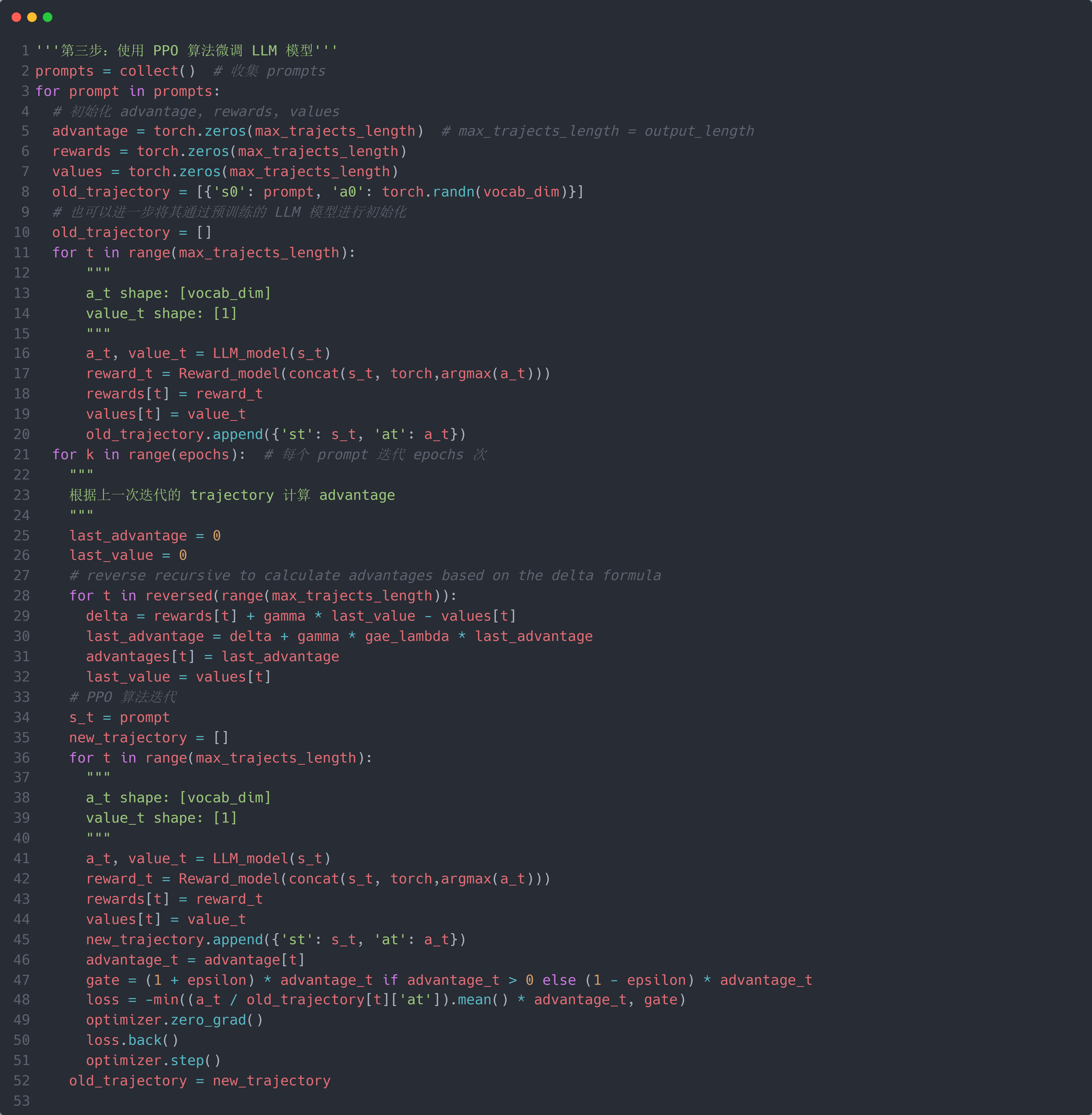
第三步：使用 PPO 算法微调 LLM 模型 $M_\theta$：首先，需要将微调(FT)问题转化为强化学习(RL)问题：预训练好的 LLM 模型 $M_\theta$ 称为 policy model $\pi_\theta(a|s)$ (它每次输出一个词)；预训练好的奖励模型 $r_\theta$ 称为 reward model $r_\theta(s, a)$. 而文本数据称为状态(state) $s$，则输入的文本数据 $x$ 称为初始状态 $s_0$；一个词称为动作(action) $a$. 所以，初始时 policy model 为 $\pi_{\theta_0}(\cdot)$，state 为 $s_0$，将状态 $s_0$ 输入 $\pi_{\theta_0}(\cdot)$ 得到预测的 action $a_0 = \pi_{\theta_0}(a_0|s_0)$，然后将 $a_0$ 拼接到状态 $s_0$ 后面生成新 state $s_1$，并将新 state $s_1$ 模型 $\pi_{\theta_0}(\cdot)$ 生成新 action $a_1$. 如此循环往复生成 policy model $\pi_{\theta_0}(\cdot)$ 预测的 trajectory $\{(s_0, a_0), ..., (s_m, a_m)\}$ (这不就是 LLM 模型的 predict-next-token 的方式嘛😀，所以 $\pi_{\theta_0}(\cdot)=M_\theta$，$a_i = y_i$，$s_i = concat(x,y_{[1:i-L_I]})$，$m=L_O$，就是为了对齐 PPO 算法换了个名字而已. 注意：是每个词是一个 action，而不是一个 $y$ 是一个 action，不要和第二步排序混淆了(我就搞混了😟)).

题外话：这段话实属经典，建议反复阅读来理解如何将 FT 问题转化为 RL 问题(from hf blog)：First, the policy is a language model that takes in a prompt and returns a sequence of text (or just probability distributions over text). The action space of this policy is all the tokens corresponding to the vocabulary of the language model (often on the order of 50k tokens) and the observation space is the distribution of possible input token sequences, which is also quite large given previous uses of RL (the dimension is approximately the size of vocabulary $\times$ length of the input token sequence). The reward function is a combination of the preference model and a constraint on policy shift.

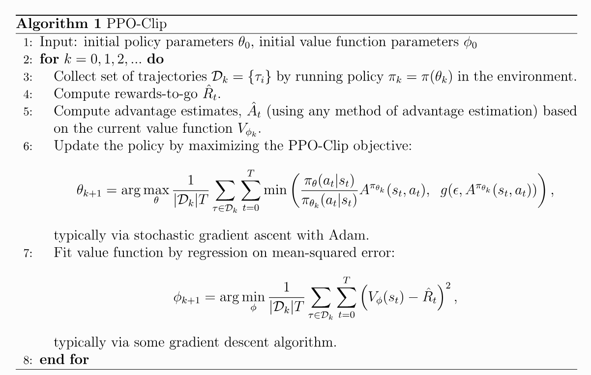
下一步就是构造 PPO 的优化函数来训练 policy model $\pi_\theta(a|s)$. 注意，接下来的 PPO 都是以一个 trajectory 为一个迭代总体(类似 epoch)，以一个 $(s, a)$ 为一次迭代基元(类似 item)，因此下文中的 $t \in \{1, ..., m\}$. 如上图所示，原始的 PPO 优化函数为：

其中 $\pi_{\theta_{\mathrm{old}}}(a_t\mid s_t)$ 表示之前迭代的 policy model (可能来自前一轮 epoch，也可能就是初始化的)；$\pi_\theta(a_t\mid s_t)$ 表示目前正在迭代的 policy model；$r_t(\theta)$ 表示之前的 policy model 和目前的 policy model 的输出的差异(用比值来衡量)；而 $\operatorname{clip}(r_t(\theta),1-\epsilon,1+\epsilon)$ 表示将 $r_t(\theta)$ 的值限制在 $(1-\epsilon,1+\epsilon)$ 之间来保证 policy model 更新迭代的变化不能过大(即不能偏离 $\pi_{\theta_{\mathrm{old}}}(a_t\mid s_t)$ 的分布太多，有点 smooth-update 的思想). $\hat{A}_t$ 表示 Advantage，用于衡量当前预测的 action $a_t$ 得到的 reward 是否比其他所有可能的 action 的平均 reward 要高：如果是，则 $\hat{A}_t > 0$；反之，则 $\hat{A}_t < 0$. 其计算公式为：

题外话：想要了解 PPO 的优化函数的具体推导过程及其每个表达式的含义，可以参考 huggingface blog.

可以看到，$\hat{A}_t$ 的计算是从后往前推的，它需要先计算出整个 trajectory；因此，$\hat{A}_t$ 的计算是基于上一次迭代生成的 trajectory：假设上一次迭代的 trajectory 为 $\{(s_0, a_0, V(s_0)), ..., (s_m, a_m, V(s_m))\}$，然后通过上述计算公式得到 $\hat{A} = {\hat{A}_m, ..., \hat{A}_0}$，然后将 $\hat{A}$ 输入到下一次迭代进行优化函数值的计算.

接下来，将原始的 PPO 优化函数中的每个部分都对应到微调 LLM 上(其实也只有 $V(\cdot)$ 和 $L^{CLIP}(\theta)$ 略有差异). 在前述中，我们提到通常将 policy $\pi_\theta(\cdot)$，reward $r$ 和 value $V(\cdot)$ 都建模为 NN 模型 $\pi_\theta(a|s)$，$r_\theta(s, a)$ 和 $V_\theta(s)$. 现在我们已经实现了 $\pi_\theta(a|s)$，$r_\theta(s, a)$，那么 $V_\theta(\cdot)$ 如何实现？很简单，只需要在 $\pi_\theta(a|s)$ (即 Transformer Decoder)的最后再并行增加一个线性回归 MLP，使其预测连续值 $v \in \mathbb{R}$ 即可；而这个 MLP 的参数是随机初始化的(所以第三步中的所有 $V(\cdot) = V_\theta(\cdot)$). 因此 $\pi_\theta(\cdot)$ 和 $V_\theta(\cdot)$ 共享大部分参数. 同时，$\pi_{\theta_{\mathrm{old}}}(\cdot)$ 不是采用上一次迭代的 policy model，而是直接采用初始化的 policy model $\pi_{\theta_{0}}(\cdot)$，并对其做了进一步简化，最终得到(其中 $k$ 表示第 $k$ 次迭代总体(即第 $k$ 个 epoch))：

RLHF 的具体(简易)代码

simple pesudocode

References

1. Illustrating Reinforcement Learning from Human Feedback (RLHF)

2. Proximal Policy Optimization (PPO)

3. Implementing RLHF with Custom Datasets

4. Coding chatGPT from Scratch Lecture 2: PPO Implementation

5. PPO_Implementation.ipynb

6. Coding chatGPT from Scratch Lecture 1: PPO Theory

7. RLHF (Reinforcement Learning From Human Feedback): Overview + Tutorial

8. The N Implementation Details of RLHF with PPO

9. The 37 Implementation Details of Proximal Policy Optimization

10. Approximating KL Divergence

11. RL — Proximal Policy Optimization (PPO) Explained

12. Elo rating system